
No Free Lunch Theorem (NFL)
Before we dive into the algorithms for the creation of models about the data, we need some foundations. The first foundation is a fundamental theorem about optimization algorithms, the No Free Lunch Theorem (NFL). This now gets a bit theoretical, if you are just interested in the (very important!) consequences of the theorem on data modeling, just skip to the colloquial definition. The mathematical formulation of the NFL is the following.
No Free Lunch Theorem:
Let $d_m^y$ be ordered sets of size $m$ with cost values $y \in Y$. Let $f: X \to Y$ a function that should be optimized. Let $P(d_m^y|f, m, a)$ the conditional probability of getting $d_m^y$ by $m$ times running the algorithm $a$ on the function $f$.
For any pair of algorithms $a_1$ and $a_2$ to following equations holds:
$$\sum_f P(d_m^y|f, m, a_1) = \sum_f P(d_m^y|f, m, a_2)$$
A proof for the theorem can be found in the literature. The equation of the NFL tells us the sum of the probabilities of getting certain costs is equal if all functions $f$ are considered for any two algorithms. The meaning of this can be summarized as follows.
No Free Lunch Theorem (Colloquial):
All algorithms are equal when all possible problems are considered.
This is counter-intuitive, because we observe notable differences between different algorithms in practice. However, the NFL does not prohibit that an algorithm is better for some functions $f$ - i.e., for some problems. But if an algorithm is better than the average algorithm for some problems, the NFL tells us that the algorithm must be worse than the average algorithm for other problems. Thus, the true consequence of the NFL is that there is not one algorithm that is optimal for all problems. Instead, different algorithms are better for different problems. That is also the reason for the name: there is no "free lunch", i.e., one algorithm for all problems. Instead, data scientists must earn their lunch, i.e., find a suitable algorithm.
This means that having detailed knowledge about one algorithm is not sufficient. Data scientists need a whole toolbox of algorithms. They must be able to select a suitable algorithm, based on the data, their knowledge about the problem, and their experience based on working with different algorithms. Over time, data scientists gather experience with more and more algorithms and become experts in selecting suitable algorithms for a given problem.
Definition of Machine Learning
Machine learning is currently one of the hottest topics in computer science because recent advances in using the growth of computational power and the available data have led to vast improvements for hard problems, e.g., object recognition, automated translation of languages, and playing games.
To get started with machine learning, we must first understand the meaning of the term. There are many definitions out there. Tom Mitchel gave a very powerful and versatile definition of machine learning:
Definition of Machine Learning:
A computer program is said to learn from experience $E$ with respect to some class of tasks $T$ and performance measure $P$, if its performance at tasks $T$, as measured by $P$, improves with experience $E$.
At the first glance this definition looks very abstract and the sentence is hard to parse, especially because of the usage of the abstract terms of experience, tasks, and performance measures. However, this is exactly what makes this definition so good: it actually fits the versatile field of machine learning. To understand the definition, we just need to understand what is meant with experience, task, and performance measure.
- The experience is (almost always) our data. The more data we have, the more experience we have. However, there are also self-learning systems that do not require data but generate their own experience, like AlphaZero that learns just by playing against itself, i.e., not from data of prior games. In this case, the experience is gained by playing more and more games.
- The tasks are what we want to solve. You want to recognize pedestrians so that your self-driving car does not run them over? You want to play and win games? You want to make users click on links of advertisements? Those are your tasks. In general, the task is closely related to your use case and the business objective. In a more abstract way, these tasks can be mapped to generic categories of algorithms, which we discuss later.
- The performance measure is an estimate of how good you are at the tasks. Performance measures may be the numbers of pedestrians that are correctly identified and the number of other objects that are mistakenly identified as pedestrians, the number of games that are won, or the number of clicks on advertisements.
With this in mind, the definition is suddenly clear and simple: We just have programs that get better at their tasks with more data.
Features
Before we start to look at algorithms for machine learning in the next chapters, we first establish some basic concepts. At the foundation of machine learning we have features. The meaning of features is best explained using an example. As humans, we immediately know that the following picture shows a whale.

How exactly humans recognize objects is still a matter of research. However, let us assume we identify what different parts of the picture are and then know what the complete picture is about by combining these parts. For example, we might see that there is a roughly oval shaped object in the foreground, that is black on top and white on the bottom, that has fins and is in front of a mostly blue background. We can describe the picture using this information as features.
This is what machine learning is about: reasoning about objects by representing them as features. Formally, we have an object space $O$ with real-world objects and a feature space $\mathcal{F}$ with descriptions of the objects. A feature map $\phi: O \to \mathcal{F}$ maps the objects to their representation in the feature space.
For our whale picture, the object space $O$ would be pictures and the feature space $\mathcal{F}$ would have five dimensions: shape, top color, bottom color, background color, has fins. The feature representation of the whale picture would be $\phi(whale picture) = (oval, black, white, blue, true)$.
There are different types of features, which can be categorized using Steven's levels of measurement into the NOIR schema based on the scale that they are using: nominal, ordinal, interval, and ratios.
| Scale | Property | Allowed Operations | Example |
|---|---|---|---|
| Nominal | Classification or membership | $=, \neq$ | Color as black, white, and blue |
| Ordinal | Comparison of levels | $=, \neq, >, <$ | Size in small, medium, and large |
| Interval | Differences of affinities | $=, \neq, >, <, + ,-$ | Dates, temperatures, discrete numeric values |
| Ratio | Magnitudes or amounts | $=, \neq, >, <, +, -, *, /$ | Size in cm, duration in seconds, continuous numeric values |
The nominal and ordinal features are also known as categorical features. For nominal features, we only have categories, but cannot establish which category is larger or which categories are closer to each other. For ordinal features, we can establish an order between the categories, but we do not know the magnitude of the differences between the categories. Thus, while we may know that small is smaller than medium and that medium is smaller than large, we do not know which difference is larger. This is what we get with interval scales. With features on interval scales we can quantify the size of differences. However, we cannot directly establish by which ratio something changed. For example, we cannot say that the date 2000-01-01 is twice as much as the date 1000-01-01. For this, we need a ratio scale. For example, if we measure the difference in year to the year 0 in the Gregorian calendar, we can say that 2000 years difference is twice as much as 1000 years.
Many machine learning algorithms require that features must be represented numerically. While this is the native representation of features on interval and ratio scales, nominal and ordinal features are not numeric. A naive approach would be to just assign each category a number, e.g, black is 1, white is 2, blue is 3. This naive approach is very dangerous because it would be possible for algorithms to, e.g., calculate the difference between black and white as 2, which does not make sense at all. A better solution is to use a one-hot encoding. The concept behind the one-hot encoding is to expand a nominal/ordinal scale into multiple nominal scales with the values 0 and 1. Each category of the original scale gets its own expanded scale, the value of the new feature is 1, if an instance is of that category, and 0 otherwise.
For example, consider a feature with a nominal scale with values black, white and blue, i.e., $x \in \{black, white, blue\}$. We expand this feature into three new features, i.e., $x^{black}, x^{white}, x^{blue} \in \{0,1\}$. The values of the new features are: $$x^{black} = \begin{cases}1 & \text{if}~x=\text{black} \\ 0 & \text{otherwise}\end{cases}$$ $$x^{white} = \begin{cases}1 & \text{if}~x=\text{white} \\ 0 & \text{otherwise}\end{cases}$$ $$x^{blue} = \begin{cases}1 & \text{if}~x=\text{blue} \\ 0 & \text{otherwise}\end{cases}$$
With the approach above, we need $n$ new categories, if the scale of our original feature has $n$ distinct values. In the example above, we have three new features for a scale with three values. It is also possible to use one-hot encoding with $n-1$ new features. We could just leave out $x^{blue}$ from our example and still always know when the value would have been blue: when it is neither black nor white, i.e., when $x^{black}=x^{white}=0$. This is especially useful to convert scales with exactly two values. Please note that while one-hot encoding is a useful approach, it does not work well if you have lots of categories, because a lot of new features are introduced. Moreover, the order of ordinal features is lost, i.e., we loose information when one-hot encoding is used for ordinal features.
Training and Test Data
Data is at the core of data science. For us, data consists of instances with features. Instances are representations of real-world objects through features. The table below shows an example of data.
| shape | top color | bottom color | background color | has fins |
|---|---|---|---|---|
| oval | black | black | blue | true |
| rectangle | brown | brown | green | false |
| ... | ... | ... | ... | ... |
Each line in the table is an instance, each column contains the values of the features of that instance. Often, there is also a property you want to learn, i.e., a value of interest that is associated with each instance.
| shape | top color | bottom color | background color | has fins | value of interest |
|---|---|---|---|---|---|
| oval | black | black | blue | true | whale |
| rectangle | brown | brown | green | false | bear |
| ... | ... | ... | ... | ... | ... |
Depending on whether this value is known and may be used for the creation of models, we distinguish between supervised learning and unsupervised learning. Examples for both supervised and unsupervised algorithms are discussed here.
Data is often organized in different sets of data. The most frequently used terms are training data and test data. Training data is used for the creation of models, i.e., for everything from the data exploration, the determination of suitable analysis approaches, as well as experiments with different models to select the best model. You may use your training data as often as possible and transform the data however you like.
In an ideal world, the test data is only used one time, i.e., once you have finished the model building and want to determine how well your model would perform in a real-world estimation. The model you created is then executed against the test data and you evaluate the performance of that model with the criteria you determined in the discovery phase.
The strong differentiation between training and test data is to prevent overfitting and evaluate how your results generalize. Overfitting occurs, when data is memorized. For example, we can easily create a model that perfectly predicts our training data: we just memorize all instances and predict their exact value. However, this model would not work at all on other data. Therefore, it would be useless on all other data. This is why we have test data: this data was never seen during the creation of the model. If our model is good and actually does what it is supposed to do, it should also perform well on the test data.
Unfortunately, data is often limited and the creation of more data can be difficult or expensive. On the one hand, we know that machine learning algorithms yield better results with more data. On the other hand, the performance estimate on the test data is also more reliable, if we have more test data. Therefore, how much data is used as training data and how much data is as test data is a tradeoff that must be decided in every project. The best approach is to use hold-out data. This is real test data that is only used once. Common ratios between training and test data are, e.g.,
- 50% training data, 50% test data.
- 66.6% training data, 33.4% test data.
- 75% training data, 25% test data.
Sometimes, there are additional concerns to consider. First, there is something called validation data. Validation data is "test data for training models". This means that the data is used in the same way the test data is used at the end of the project, but may be used repeatedly during the creation of models. Validation data can, e.g., be used to compare different models to each other and select the best candidate. Validation data can be created as hold-out data as well, e.g., with 50% training data, 25% validation data, and 25% test data.
In case there is not enough data, cross-validation may be used to prevent overfitting of models. With cross-validation, there is no clear separation of training and test data. Instead, all data is used for training and testing of the models. With $k$-fold cross-validation, the data is split into $k$ partitions of equal sizes. Each partition is once used for testing, the other partitions are used for the training.
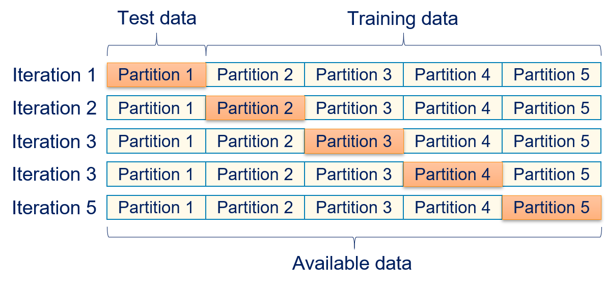
The performance is then estimated as the mean of the results of the testing on each partition. With cross-validation, each instance in the data is used as test data exactly once. The drawback of cross-validation is that there is no real test data. Instead, what we called test data - because that is the common terminology in the literature with respect to cross-validation - is actually only validation data. Thus, cross-validation may not detect all types of overfitting and tends to overestimate the performance of models. Thus, you should use hold-out data whenever possible.
Categories of Algorithms
Depending on the data and the use case, there are different categories of algorithms that may be suitable.
- Association rule mining is about finding relationships between items in transactions. The most common use case is the prediction of items, which may be added to a shopping basket, based on items that are already within the basket. We cover the Apriori algorithm for association rule mining in Chapter 5.
- Clustering is about finding groups of similar items, respectively the identification of instances that are structurally similar. Both problems are the same because groups of similar items can be inferred by finding structurally similar items. We cover $k$-means clustering, EM clustering, DBSCAN, and single linkage clustering in Chapter 6.
- Classification is about the assignment of labels to objects. We cover the $k$-nearest neighbor algorithm, decision trees, random forests, logistic regression, naive bayes, support vector machines, and neural networks in Chapter 7.
- Regression is about the relationship between features, possibly with the goal to predict numeric values. We cover linear regression with ordinary least squares, ridge, lasso, and the elastic net in Chapter 8.
- Time series analysis is about the the analysis of temporal data, e.g., daily, weekly, or monthly data. Time series analysis goes beyond regression, because aspects like the season are considered. We cover ARIMA in Chapter 9.
- Text mining of unstructured textual data. All approaches above may be applied to text, once a structure has been imposed. We cover a basic bag-of-words approach for text mining in Chapter 10.
Association rule mining and clustering are examples for unsupervised learning. Both work only based on patterns within the data without any guidance by a value of interest. Hence, such approaches are also called pattern recognition. Classification, regression, and time series analysis are examples for supervised learning. These approaches work based on learning how known values can be correctly learned from the values of features.