
Overview
Associations are relationships between objects. The idea behind association rule mining is to determine rules, that allow us to identify which objects may be related to a set of objects we already know. In the association rule mining terminology, we refer to the objects as items. A common example for association rule mining is basket analysis. A shopper puts items from a store into a basket. Once there are some items in the basket, it is possible to recommend associated items that are available in the store to the shopper.
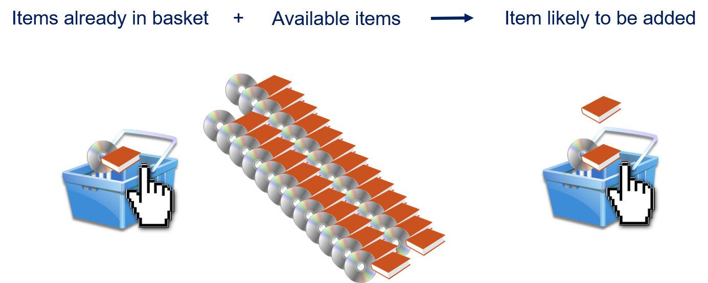
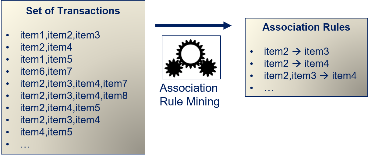
In this example, the association between items is defined as "shoppers bought items together". More generally speaking, we have transactions, and in each transaction we observe a set of related objects. We apply association rule mining to a set of transactions to infer association rules that describe the associations between items.
The relationship that the rules describe should be "interesting". The meaning of interesting is defined by the use case. In the example above, interesting is defined as "shoppers bought items together". If the association rules should, e.g., find groups of collaborators, interesting would be defined as "worked together in the past".
We can also formally define association rule mining. We have a finite set of items $I = \{i_1, ..., i_m\}$ and transactions that are a subset of the items, i.e., transactions $T = \{t_1, ..., t_n \}$ with $t_j \subseteq I, j=1, ..., n$. Association rules are logical rules of the form $X \Rightarrow Y$, where $X$ and $Y$ are disjoint subsets of items, i.e., $X, Y \subseteq I$ and $X \cap Y = \emptyset$. We refer to $X$ as the antecedent or left-hand-side of the rule and to $Y$ as the consequent or right-hand-side of the rule.
Note:
You may notice that we do not speak of features, but only of items. Moreover, we do not speak of instances, but rather of transactions. The reason for this is two-fold. First, this is the common terminology with respect to association rule mining. Second, there are no real features, the objects are defined by their identity. The transactions are the same as the instances from Chapter 4.
The goal of association rule mining is to identify good rules based on a set of transactions. A generic way to define "interesting relationships" is that items occur often together in transactions. Consider the following example with ten transactions.
# we define each transaction as a list
# a set of transactions is a list of lists
data = [['item1', 'item2', 'item3'],
        ['item2', 'item4'],
        ['item1', 'item5'],
        ['item6', 'item7'],
        ['item2', 'item3', 'item4', 'item7'],
        ['item2', 'item3', 'item4', 'item8'],
        ['item2', 'item4', 'item5'],
        ['item2', 'item3', 'item4'],
        ['item4', 'item5'],
        ['item6', 'item7']]
data
We can see that the items item2, item3, and item4 occur often together. Thus, there seems to be an interesting relationship between the items. The question is, how can we find such interesting combinations of items automatically and how can we create good rules from interesting combinations of items.
The Apriori Algorithm
The Apriori algorithm is a relatively simple, but also powerful algorithm for finding associations.
Support and Frequent Itemsets
The algorithm is based on the concept of the support of itemsets $IS \subseteq I$. The support of an itemset $IS$ is defined as the ratio of transaction in which all items $i \in IS$ occur, i.e., $$support(IS) = \frac{|\{t \in T: IS \subseteq t\}|}{|T|}.$$
The support mimics our generic definition of interesting from above, because it directly measures how often combinations of items occur. Thus, support is an indirect measure for interestingness. What we are still missing is a minimal level of interestingness for us to consider building rules from an itemset. We define this using a minimal level of support that is required for an itemset. All itemsets that have a support greater than this threshold are called frequent itemset. Formally, we call an itemset frequent $IS \subset I$, if $support(IS) \geq minsupp$ for a minimal required support $minsupp \in [0,1]$.
In our example above, the items item2, item3, and item4 would have $support(\{item2, item3, item4\}) = \frac{3}{10}$, because all three items occur together in three of the ten transactions. Thus, if we use $minsupp=0.3$, this we would call $\{item2, item3, item4\}$ frequent. Overall, we find the following frequent itemsets.
# we need pandas and mlxtend for the association rules
import pandas as pd
from mlxtend.frequent_patterns import apriori
from mlxtend.preprocessing import TransactionEncoder
pd.set_option('styler.render.repr', 'latex')

# we first need to create a one-hot encoding of our transactions
te = TransactionEncoder()
te_ary = te.fit_transform(data)
data_df = pd.DataFrame(te_ary, columns=te.columns_)

# we can use this function to determine all itemsets with at least 0.3 support
# what apriori is will be explained later
frequent_itemsets = apriori(pd.DataFrame(data_df), min_support=0.3, use_colnames=True)
frequent_itemsets
Deriving Rules from Itemsets
A frequent itemset is not yet an association rule, i.e., we do not have an antecedent $X$ and a consequent $Y$ to create a rule $X \Rightarrow Y$. There is a simple way to create rules from a frequent itemset. We can just consider all possible splits of the frequent itemset in two partitions, i.e, all combinations $X, Y \subseteq IS$ such that $X \cup Y = IS$ and $X \cap Y = \emptyset$.
This means we can derive eight rules from the itemset $\{item2, item3, item4\}$:
from mlxtend.frequent_patterns import association_rules

association_rules(frequent_itemsets.iloc[8:9, :], metric="confidence",
                  min_threshold=0.0, support_only=True)[['antecedents', 'consequents']]
The two remaining rules use the empty set as antecedent/consequent, i.e.,
- $\emptyset \Rightarrow \{item2, item3, item4\}$
- $\{item2, item3, item4\} \Rightarrow \emptyset$
Since these rules to not allow for any meaningful associations, we ignore them.
Confidence, Lift, and Leverage
An open question is how we may decide if these rules are good or not. Thus, we need measures to identify if the associations are meaningful or if they are just the result of random effects. This cannot be decided based on the support alone. For example, consider a Web shop with free items. These items are likely in very many baskets. Thus, they will be part of many frequent itemsets. However, we cannot really conclude anything from this item, because it is just added randomly because it is free, not because it is associated with other items. Moreover, the support of a rule $X \Rightarrow Y$ is always the same as for the rule $Y \Rightarrow X$. However, there may be differences, because causal associations are often directed. The measures of confidence, lift, and leverage can be used to see if a rule a is random or if there is really an association.
The confidence of a rule is defined as
$$confidence(X \Rightarrow Y) = \frac{support(X \cup Y)}{support(X)},$$i.e. the confidence is the ratio of observing the antecedent and the consequent together in relation to only the transactions that contain $X$. A high confidence indicates that the consequent often occurs when the antecedent is in a transaction.
The lift of a rule is defined as
$$lift(X \Rightarrow Y) = \frac{support(X \cup Y)}{support(X) \cdot support(Y)}.$$The lift measures the ratio between how often the antecedent and the consequent are observed together and how often they would be expected to be observed together, given their individual support. The denominator is the expected value, given that antecedent and consequent are independent of each other. Thus, a lift of 2 means, that $X$ and $Y$ occur twice as often together, as would be expected if there was no association between the two. If the antecedent and the consequent are completely independent of each other, the lift is 1.
The leverage of a rule is defined as
$$leverage(X \Rightarrow Y) = support(X \cup Y) - support(X) \cdot support(Y).$$This definition is almost the same as for the lift, except that the difference is used instead of the ratio. Thus, there is a close relationship between lift and leverage. In general, leverage slightly favors itemsets with larger support.
To better understand how the confidence, lift, and leverage work, we look at the values for the rules we derived from the itemset $\{item2, item3, item4\}$.
# all rules for our data
# we drop the column conviction, because this metric is not covered here
# we also drop all rules from other itemsets than above.
association_rules(frequent_itemsets, metric="confidence",
                  min_threshold=0.0).drop('conviction', axis=1)[6:].reset_index(drop=True)
Based on the metrics, the best rules seem to be $\{item3, item4\} \Rightarrow \{item2\}$. This rule has a perfect confidence of 1, i.e., item2 is always present when item4 and item3 are also present. Moreover, the lift of 1.66 indicates that this is 1.66 times more often than expected. The counterpart to this rule is $\{item2\} \Rightarrow \{item3, item4\}$. The rule has the same lift, but the confidence is only 0.5. This means that item2 appears twice as often alone, as together with the items item3 and item4. Thus, we can estimate that this rule would be wrong about 50% of the time.
The best rule with a single item as antecedent is $\{item3\} \Rightarrow \{item2, item4\}$ with a confidence of 0.75 and a lfit of 1.5. Thus, in 75% of the transactions in which item3 occurs, the items item2 and item4 are also present, which is 1.5 times more often than expected.
The example also shows some general properties of the measures. Most importantly, lift and leverage are the same, if antecedent and consequent are switched, same as the support. Thus, confidence is the only measure we have introduced that takes the causality of the associations into account. We can also observe that the changes in lift and leverage are similar. The lift has the advantage that the values allow a straight forward interpretation.
Exponential Growth
We have now shown how we can determine rules: we need to find frequent itemsets and can then derive rules from these sets. Unfortunately, finding the frequent itemsets is not trivial. The problem is that the number of itemsets grows exponentially with the number of items. The possible itemsets are the powerset $\mathcal{P}$ of $I$, which means there are $|\mathcal{P}(I)|=2^{|I|}$ possible itemsets. Obviously, there are only very few use cases, where we would really need to consider all items, because often shorter rules are preferable. Unfortunately, the growth is still exponential, even if we restrict the size. We can use the binomial coefficient
$${|I| \choose k} = \frac{|I|!}{(|I|-k)!k!}$$to calculate the number of itemsets of size k. For example, if we have |I|=100 items, there are already 161,700 possible itemsets of size $k=3$. We can generate eight rules for each of these itemsets, thus we already have 1,293,600 possible rules. If we ignore rules with the empty itemset, we still have 970,200 possible rules.
Thus, we need a way to search the possible itemsets strategically to deal with the exponential nature, as attempt to find association rules could easily run out of memory or require massive amounts of computational resources, otherwise.
The Apriori Property
Finally, we come to the reason why this approach is called the Apriori algorithm.
Apriori Property
Let $IS \subseteq I$ be a frequent itemset. All subsets $IS' \subseteq IS$ are also frequent and $support(IS') \geq support(IS)$.
This property allows us to search for frequent itemsets in a bounded way. Instead of calculating all itemsets and then checking if they are frequent, we can grow frequent itemsets. Since we know that all subsets of a frequent itemset must be frequent, we know that any itemset that contains a non-frequent subset cannot be frequent. We use this to prune the search space as follows.
- Start with itemsets of size $k=1$.
- Drop all itemsets that do not have the minimal support, so that we only have frequent itemsets left.
- Create all combinations of the currently known frequent itemsets of size $k+1$
- Repeat steps 2 and 3 until
- No frequent itemsets of length $k+1$ are found
- A threshold for $k$ is reached, i.e., a maximal length of itemsets.
This algorithm can still be exponential. For example, if all transactions contain all items, all possible itemsets are frequent and we still have exponential growth. However, in practice this algorithm scales well, if the support is sufficiently high.
For example, let us consider how we can grow frequent itemsets with $minsupp=0.3$ for our example data. Here is the data again.
data
We start by looking at the support of the individual items:
| Itemset with $k=1$ | support | Drop |
|---|---|---|
| $\{item1\}$ | 0.2 | x |
| $\{item2\}$ | 0.6 | |
| $\{item3\}$ | 0.4 | |
| $\{item4\}$ | 0.5 | |
| $\{item5\}$ | 0.3 | |
| $\{item6\}$ | 0.2 | x |
| $\{item7\}$ | 0.3 | |
| $\{item8\}$ | 0.1 | x |
Since the items item1, item6, and item8 do not have the minimal support, we can drop them and do not need to consider them when we go to the itemsets of size $k=2$.
| Itemset with $k=2$ | support | Drop |
|---|---|---|
| $\{item2, item3\}$ | 0.4 | |
| $\{item2, item4\}$ | 0.5 | |
| $\{item2, item5\}$ | 0.1 | x |
| $\{item2, item7\}$ | 0.1 | x |
| $\{item3, item4\}$ | 0.3 | |
| $\{item3, item5\}$ | 0.0 | x |
| $\{item3, item7\}$ | 0.1 | x |
| $\{item4, item5\}$ | 0.2 | x |
| $\{item4, item7\}$ | 0.1 | x |
| $\{item5, item7\}$ | 0.0 | x |
As we can see, only the combinations with the items item2, item3, and item4 are frequent, all others can be dropped. This leaves is with a single combination for $k=3$.
| Itemset with $k=3$ | support | Drop |
|---|---|---|
| $\{item2, item3, item4\}$ | 0.3 |
There are no combinations of length $k=4$ possible and we are finished. We only had to evaluate the support for $8+10+1=19$ itemsets to find all frequent itemsets among all possible $2^8=256$ itemsets, i.e., we could reduce the effort by about 93% by exploiting the Apriori property and growing the itemsets.
Restrictions for Rules
So far, we always consider all possible combinations of antecedent and consequent as rules, except rules with the empty itemset. Another common restriction is to only consider rules with a single item as consequent. The advantage of such rules is that they have a higher confidence than other combinations. This means that the associations are usually strong and, consequently, more often correct.
Evaluating Association Rules
The final question that we have not yet answered is how we can determine if the associations rules we determined are good, i.e., if we found real associations and not random rules. The confidence, lift, and leverage already support this and if these measures are used in combination they are a good tool to identify rules. Confidence tells you if the relationship may be random, because the antecedent occurs very often, lift and leverage can tell you if the relationship is coincidental.
However, there are additional ways to validate that the association rules are good. For example, you can split your data into training and test data. You can then evaluate how often the associations you find in the training data also appear in the test data. If there is a big overlap, the association rules are likely good. You can also go one step further and remove items from transaction in the test data and see if your rules can predict the missing items correctly.
Finally, association rule mining is a typical example of a problem where you can achieve decent results with full automation, but likely require manual intervention to achieve very good results. Just think back to a strange recommendation you may have seen in a Web shop at some point. This was likely because there was no manual validation of the rules and the result of strange buying behavior of single customers. This can be further improved, e.g., through manual inspection of rules and filtering the automatically inferred rules. However, this is not a task for the data scientist alone, but should be supported by domain experts. The goal is to determine for the rules if the associations really make sense and only use the valid rules.